About the ECMWF db
The database use to sample the large scale fields is based on the ECMWF ensemble reforecasts. Twice a week, the ECMWF reruns their current operational model for a number of past days. In particular, on January 16th 2017, the model was rerun for all January 16th's from 1997 to 2016. Instead of a full ensemble, only 5 members are run.
The database has the following variables:
| Variable | units |
|---|---|
| 2m temperature | K |
| Precipitation | mm |
| Sea level pressure | Pa |
| Cloud area fraction | 0-1 |
| Zonal wind speed | m/s |
| Meridional wind speed | m/s |
| Incoming solar radiation | W/m2 |
These are all daily averages, except precipitation, which is a daily total.
For some forecast parameters, the model has a climatology that varies with leadtime. That is, the first day of the forecast could be dryer or wetter on average than the other forecast days. In addition, the first day may have greater or less spread of possible states than the other days.
This can be problematic for two reasons:
- The "truth" dataset (i.e. the first day of the forecasts) will have a different climatology than the simulation
- The end states of a 10-day trajectory can end up in a state that is rare for the beginning state, thereby incorrectly sampling the distribution.
To fix this, a quantile mapping correction has been applied to each leadtime. That is, leadtimes 1-9 have been adjusted such that they have the same frequency of values as leadtime 0. This proceedure is done separately on every gridpoint. Currently, we have not done this separately for each season.
The raw data in the database does not include incoming solar radiation. We diagnose this value by using a simple model that is the advantage of providing a realistic value that is consistent with the cloud cover in use.
The model is based on the articles by Sozzi et al. (2002) and Holtslag and Van Ulden (1985). The incoming solar radiation at ground level in the presence of clouds (RG, unit W/m^2) is modelled as:
RG = RG0 * (1 + b1 * TC^b2 )
where: RG0 is the incoming solar radiation under clear skies; TC is the total cloud cover (e.g. simulated by the weather generator); b1 and b2 are empirical coefficients, which may depend on the specific region considered.
The parametrization used for RG0 depends on the (refracted) solar elevation angle S:
RG0 = a1 * sin(S) * exp[-0.057/sin(S)]
If sin(S) is less than a minimum value equal to (-a2/a1), with a2=-69 W/m^2 (Holtslag and Van Ulden ,1985), then RG is set to 0 W/m^2.
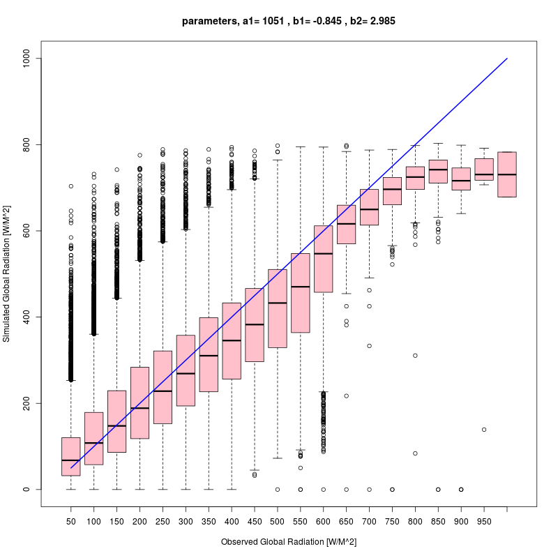
A total of three empirical coefficients need to be estimated within our diagnostic model: a1, b1, b2. The coefficients have been optimized so to better fit the incoming solar radiation measurements available in the Climate database of the Norwegian Meteorological Institute. In particular: all the stations have been considered; the measurements at the hourly time step have been used; the time period considered ranges from 01.01.2014 to 12.31.2016. The total cloud cover used to obtain the modelled RG is the one simulated by the ECMWF model, specifically we have considered the daily averaged cloud cover, as this is the variable provided by the weather generator to the users. For example, suppose January 1st 2014 at a grid point has a daily averaged cloud cover of 0.4, then a cloud cover of 0.4 has been attributed to the 24 hours of January 1st 2014. The same operation has been done for all the days/hours between 01.01.2014 and 31.12.2016 and the total cloud cover has been extracted from the gridded dataset at the station points with hourly time steps. Then, the RG modelled values have been obtained as described above and they have been compared with the observed values. The optimization of a1, b1 and b2 has been done by using a maximum likelihood method. The optimal parameter values are reported in the table:
| coefficients | value | units |
|---|---|---|
| a1 | 1051 | W/m^2 |
| b1 | -0.845 | - |
| b2 | 2.985 | - |
References:
- Sozzi R, Valentini M, Georgiadis T. Introduzione alla turbolenza atmosferica: concetti, stime, misure. Pitagora; 2002
- Holtslag AA and Van Ulden AP. Estimation of atmospheric boundary layer parameters for diffusion applications. Journal of Climate and Applied Meteorology. 1985 Nov;24(11):1196-207.