


![]()

The napari adaptation of the ImageJ/Fiji plugin AnnotatorJ for easy image annotation.
This napari plugin was generated with Cookiecutter using with @napari's cookiecutter-napari-plugin template.
Installation is possible with pip, napari or scripts.
You can install napari-annotatorj via pip:
pip install napari[all]
pip install napari-annotatorj
To install latest development version :
pip install git+https://github.com/spreka/napari-annotatorj.git
On Linux distributions, the following error may arise upon napari startup after the installation of the plugin: Could not load the Qt platform plugin “xcb” in “” even though it was found. In this case, the manual install of libxcb-xinerama0 for Qt is required:
sudo apt install libxcb-xinerama0
The bundled application version of napari allows the pip install of plugins in the .zip distribution. After installation of this release, napari-annotatorj can be installed from the Plugins --> Install/Uninstall plugins... menu by searching for its name and clicking on the Install button next to it.
Single-file install is supported on Windows and Linux (currently). It will create a virtual environment named napariAnnotatorjEnv in the parent folder of the cloned repository, install the package via pip and start napari. It requires a valid Python install.
To start it, run in the Command prompt
git clone https://github.com/spreka/napari-annotatorj.git
cd napari-annotatorj
install.bat
Or download install.bat and run it from the Command prompt.
After install, you can use startup_napari.bat to activate your installed virtual environment and run napari. Run it from the Command prompt with:
startup_napari.bat
To start it, run in the Terminal
git clone https://github.com/spreka/napari-annotatorj.git
cd napari-annotatorj
install.sh
Or download install.sh and run it from the Terminal.
After install, you can use startup_napari.sh to activate your installed virtual environment and run napari. Run it from the Terminal with:
startup_napari.sh
napari-annotatorj has several convenient functions to speed up the annotation process, make it easier and more fun. These modes can be activated by their corresponding checkboxes on the left side of the main AnnotatorJ widget.
Freehand drawing is enabled in the plugin. The "Add polygon" tool is selected by default upon startup. To draw a freehand object (shape) simply hold the mouse and drag it around the object. The contour is visualized when the mouse button is released.
See the guide below for a quick start or a demo. See shortcuts for easy operation.
-
Open --> opens an image
-
(Optionally)
- ... --> Select annotation type --> Ok --> a default tool is selected from the toolbar that fits the selected annotation type
- The default annotation type is instance
- Selected annotation type is saved to a config file
-
Start annotating objects
- instance: draw contours around objects
- semantic: paint the objects' area
- bounding box: draw rectangles around the objects
-
Save --> Select class --> saves the annotation to a file in a sub-folder of the original image folder with the name of the selected class
-
(Optionally)
- Load --> continue a previous annotation
- Overlay --> display a different annotation as overlay (semi-transparent) on the currently opened image
- Colours --> select annotation and overlay colours
- ... (coming soon) --> set options for semantic segmentation and Contour assist mode
- checkboxes --> Various options
- (default) Add automatically --> adds the most recent annotation to the ROI list automatically when releasing the left mouse button
- Smooth (coming soon) --> smooths the contour (in instance annotation type only)
- Show contours --> displays all the contours in the ROI list
- Contours assist --> suggests a contour in the region of an initial, lazily drawn contour using the deep learning method U-Net
- Show overlay --> displays the overlayed annotation if loaded with the Overlay button
- Edit mode --> edits a selected, already saved contour in the ROI list by clicking on it on the image
- Class mode --> assigns the selected class to the selected contour in the ROI list by clicking on it on the image and displays its contour in the class's colour (can be set in the Class window); clicking on the object a second time unclassifies it
- [^] --> quick export in 16-bit multi-labelled .tiff format; if classified, also exports by classes
Allows freehand drawing of object contours (shapes) with the mouse as in ImageJ.
Shape contour points are tracked automatically when the left mouse button is held and dragged to draw a shape. The shape is closed when the mouse button is released, automatically, and added to the default shapes layer (named "ROI"). In direct selection mode (from the layer controls panel), you can see the saved contour points. The slower you drag the mouse, the more contour points saved, i.e. the more refined your contour will be.
Click to watch demo video below.
Allows painting with the brush tool (labels).
Useful for semantic (e.g. scene) annotation. Currently saves all labels to binary mask only (foreground-background).
Allows drawing bounding boxes (shapes, rectangles) around objects with the mouse.
Useful for object detection annotation.
Assisted annotation via a pre-trained deep learning model's suggested contour.
- initialize a contour with mouse drag around an object
- the suggested contour is displayed automatically
- modify the contour:
- edit with mouse drag or
- erase holding "Alt" or
- invert with pressing "u"
- finalize it
- accept with pressing "q" or
- reject with pressing "Ctrl" + "Del"
- if the suggested contour is a merge of multiple objects, you can erase the dividing line around the object you wish to keep, and keep erasing (or splitting with the eraser) until the object you wish to keep is the largest, then press "q" to accept it
- this mode requires a Keras model to be present in the model folder
Click to watch demo video below
Allows to modify created objects with a brush tool.
- select an object (shape) to modify by clicking on it
- an editing layer (labels layer) is created for painting automatically
- modify the contour:
- edit with mouse drag or
- erase holding "Alt"
- finalize it
- accept with pressing "q" or
- delete with pressing "Ctrl" + "Del" or
- revert changes with pressing "Esc" (to the state before editing)
- if the edited contour is a merge of multiple objects, you can erase the dividing line around the object you wish to keep, and keep erasing (or splitting with the eraser) until the object you wish to keep is the largest, then press "q" to accept it
Click to watch demo video below
Allows to assign class labels to objects by clicking on shapes.
- select a class from the class list to assign
- click on an object (shape) to assign the selected class label to it
- the contour colour of the clicked object will be updated to the selected class colour, plus the class label is updated in the text properties of object (turn on "display text" on the layer control panel to see the text properties as
objectID:(classLabel)e.g. 1:(0) for the first object)
- optionally, you can set a default class for all currently unlabelled objects on the ROI (shapes) layer by selecting a class from the drop-down menu on the right to the text label "Default class"
- class colours can be changed with the drop-down menu right to the class list; upon selection, all objects whose class label is the currently selected class will have their contour colour updated to the selected colour
- clicking on an object that has already been assigned a class label will unclassify it: assign the label 0 to it
Click to watch demo video below
See also: Quick export
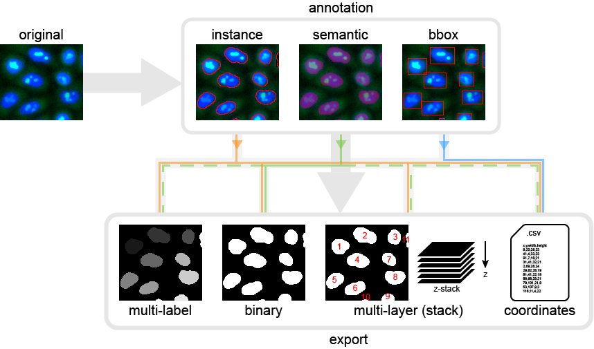
The exporter plugin AnnotatorJExport can be invoked from the Plugins menu under the plugin name napari-annotatorj. It is used for batch export of annotations to various formats directly suitable to train different types of deep learning models. See a demonstrative figure in the AnnotatorJ repository and further description in its README or documentation.
- browse original image folder with either the
- "Browse original..." button or
- text input field next to it
- browse annotation folder with either the
- "Browse annot..." button or
- text input field next to it
- select the export options you wish to export the annotations to (see tooltips on hover for help)
- at least one export option must be selected to start export
- (optional) right click on the checkbox "Coordinates" to switch between the default COCO format and YOLO format; see explanation
- click on "Export masks" to start the export
- this will open a progress bar in the napari window and close it upon finish
The folder structure required by the exporter is as follows:
image_folder
	|--- image1.png
	|--- another_image.png
	|--- something.png
	|--- ...

annotation_folder
	|--- image1_ROIs.zip
	|--- another_image_ROIs.zip
	|--- something_ROIs.zip
	|--- ...
Multiple export options can be selected at once, any selected will create a subfolder in the folder where the annotations are saved.
Click to watch demo video below
Click on the "[^]" button to quickly save annotations and export to mask image. It saves the current annotations (shapes) to an ImageJ-compatible roi.zip file and a generated a 16-bit multi-labelled mask image to the subfolder "masks" under the current original image's folder.
In the AnnotatorJExport plugin 2 coordinates formats can be selecting by right clicking on the Coordinates checkbox: COCO or YOLO. The default is COCO.
COCO format:
[x, y, width, height]based on the top-left corner of the bounding box around the object- coordinates are not normalized
- annotations are saved with header to
- .csv file
- tab delimeted
YOLO format:
[class, x, y, width, height]based on the center point of the bounding box around the object- coordinates are normalized to the image size as floating point values between 0 and 1
- annotations are saved with header to
- .txt file
- whitespace delimeted
- class is saved as the 1st column
A separate annotation file can be loaded as overlay for convenience, e.g. to compare annotations.
- load another annotation file with the "Overlay" button
- (optional) switch its visibility with the "Show overlay" checkbox
- (optional) change the contour colour of the overlay shapes with the "Colours" button
Clicking on the "Colours" button opens the Colours widget where you can set the annotation and overlay colours.
- select a colour from the drop-down list either next to the text label "overlay" or "annotation"
- click the "Ok" button to apply changes
- contour colour of shapes on the annotation shapes layer (named "ROI") that already have a class label assigned to them will not be updated to the new annotation colour, only those not having a class label (the class label can be displayed with the "display text" checkbox on the layer controls panel as
objectID:(classLabel)e.g. 1:(0) for the first object) - contour colour of shapes on the overlay shapes layer (named "overlay") will all have the overlay colour set, regardless of any existing class information saved to the annotation file loaded as overlay
The Contour assist mode imports a pre-trained Keras model from a folder named models under exactly the path napari_annotatorj. This is automatically created on the first startup in your user folder:
C:\Users\Username\.napari_annotatorjon Windows\home\username\.napari_annotatorjon Linux
A pre-trained model for nucleus segmentation is automatically downloaded from the GitHub repository of the ImageJ version of AnnotatorJ. The model will be saved to [your user folder]\.napari_annotatorj\models\model_real.h5. This location is printed to the console (command prompt or powershell on Windows, terminal on Linux).
(deprecated) When bulding from source the model folder is located at path\to\napari-annotatorj\src\napari_annotatorj\models whereas installing from pypi it is located at path\to\virtualenv\Lib\site-packages\napari_annotatorj\models.
The model must be in either of these file formats:
- config .json file + weights file: model_real.json and model_real_weights.h5
- combined weights file: model_real.hdf5
You can also train a new model on your own data in e.g. Python and save it with this code block:
	# save model as json
	model_json=model.to_json()
	with open(‘model_real.json’, ‘w’) as f:
		f.write(model_json)

	# save weights too
	model.save_weights(‘model_real_weights.h5’)
You can also train in the train widget.
This configuration will change in the next release to allow model browse and custom model name in an options widget.
To start training a new model or refine an existing one click the Train button on the right of the napari-annotatorj widget. This will open the training widget where you can set input paths and training options. During training a progress bar will show the epochs passed and plot the loss on a graph. See a guide below.
The trained model will be saved to the model folder under the located training data folder which is named training by default when preparing data. Each new training will be saved to a new training folder with increased numbering e.g. training_1, training_2 etc.
When an existing training data folder is browsed with the "Browse train ..." button, the model folder will be created under it without an additiona training folder.
After training is finished, a message is shown to indicate the newly trained model can be tested by drawing bounding boxes (rectangles) to initiate contour assist prediction. The presented region on the editing layer (Label layer) can be modified with the paint brush tool (automatically selected) as in contour assist.
The trained model can be further refined by selecting the "Retrain latest" checkbox from the training parameters (⚙ button on the right).
To use this new model for annotation in contour assist mode, you mush set the model path in the Options widget or in the configuration file (see how to here), then restart napari.
- On current annotation
- "Use current annotation" checkbox --> use this image and its current annotation for training
- Prep data --> prepare data to suitable format
- (optional) ⚙ --> set parameters
- Start --> start training
- Additional data
- Select images and annotations to use for training
- Browse original ... --> locate folder of original images
- Browse annot ... --> locate folder of annotations
- Prep data --> prepare data to suitable format
- Browse train ... --> select already prepared training data
- (optional) ⚙ --> set parameters
- Start --> start training
- Select images and annotations to use for training
The data format expected by the training widget is as follows.
images
	|--- image1.png
	|--- another_image.png
	|--- something.png
	|--- ...

unet_masks
	|--- image1.tiff
	|--- another_image.tiff
	|--- something.tiff
	|--- ...
Masks are 8-bit binary (black and white) .tiff images that can be exported from the Exporter widget selecting the Semantic (binary) export option. When the "Prep data" button is clicked in the Training widget, these folders are automatically created from the located annotation files and original images.
The following configurable parameters can be set after clicking on the ⚙ icon:
| Parameter | Description | Default value |
|---|---|---|
| Epochs | number of epochs to train | 5 |
| Steps | number of steps in each epoch | 1 |
| Batch size | number of samples in an iteration | 1 |
| Image size | size of training images | 256 |
| Start from scratch | train a new model from scratch | False |
| Retrain latest | re-fine latest training | False |
| Write pred | write test image prediction to file | False |
| Test image | path to test image | None |
Note: by default CPU will be used for training. This can be changed to GPU in the Options widget if your computer has a capable CUDA-device.
Settings found in the configuration file can be set in the Options widget opened with the "..." button on the right of the main plugin. For changes to take effect you must save your changes with the "Ok" button at the bottom of the Options widget.
The following options can be configured:
| Group | Option | Description | Default | Valid values |
|---|---|---|---|---|
| General | Annotation type | see instance, bbox, semantic | instance | instance, bbox, semantic |
| Remember annotation type | use the same annotation type on next startup | True |
True, False |
|
| Colours | select annotation and overlay colours; see here | white | white, red, green, blue, cyan, magenta, yellow, orange, black | |
| Classes | names of folders to save annotations when not classified* | normal | (any string)** | |
| Semantic segmentation | Brush size | size of the brush | 50 | int |
| Advanced settings | ||||
| Contour assist | Max distance | number of pixels to extend the initial contour with | 17 | int |
| Threshold | intensity threshold after prediction | |||
| - gray | 0.1 | float in [0,1] |
||
| - R (red) | 0.2 | float in [0,1] |
||
| - G (green) | 0.4 | float in [0,1] |
||
| - B (blue) | 0.2 | float in [0,1] |
||
| Brush size | correction brush size | 5 | int |
|
| Method | contour assist prediction method | U-Net | U-Net, Classic*** | |
| Model | U-Net model to use for Contour assist prediction | |||
| folder | path to the model folder | user/.napari_annotatorj/models |
existing models folder path |
|
| .json file | name of the model .json file without extension | model_real | any string** | |
| weights file | name of the model weights file | model_real_weights.h5 | any string** | |
| full file | name of the combined config+weights file | model_real.hdf5 | any string** | |
| Device | computation device to perform prediction | cpu | cpu,int**** |
|
| Mask/text import | ||||
| Auto mask load | load annotation files automatically when a new image is opened | False |
True, False |
|
| Enable mask load | load instance annotation mask image | False |
True, False |
|
| Enable text load | load object detection bounding box coordinate text file | False |
True, False |
|
| Method | load as editable or overlay | load | load, overlay | |
| Others | ||||
| Save outlines | save image with annotations outlined | False |
True, False |
|
| Show help on startup | show the help window upon every startup | False |
True, False |
|
| Save annot times | save annotation times to text file***** | False |
True, False |
*: right click the last element (other...) to add a new item to the list. When annotations are assigned class labels in class mode, they will be saved to the folder masks by default.
**: do not use whitespace (' ') if possible
***: region growing classical algorithm
****: valid id of a GPU device e.g. 0 or 3; if your computer has only one GPU the id is 0
*****: currently disabled, used for development
Run a demo of napari-annotatorj with sample data: a small 3-channel RGB image as original image and an ImageJ roi.zip file as annotations loaded.
    # from the napari-annotatorj folder
	python src/napari_annotatorj/load_imagej_roi.py
Alternatively, you can startup the napari-annotatorj plugin by running
    # from the napari-annotatorj folder
python src/napari_annotatorj/startup_annotatorj.py| Function | Shortcut |
|---|---|
| Contour assist | a |
| Class mode | c |
| Edit mode | Shift + e |
| Show contours | Shift + v |
| Accept Contour assist | q |
| Reject Contour assist | Ctrl + del |
| Invert Contour assist | u |
| Erase in Edit/Contour assist mode | Alt (hold) |
| Revert changes in Edit mode | Esc |
The Contour assist mode uses a pre-trained U-Net model for suggesting contours based on a lazily initialized contour drawn by the user. The default configuration loads and runs the model on the CPU so all users can run it. It is possible to switch to GPU if you have:
- a CUDA-capable GPU in your computer
- nVidia's CUDA toolkit + cuDNN installed
See installation guide on nVidia's website according to your system.
To switch to GPU utilization, edit _dock_widget.py and set to the device you would like to use. Valid values are 'cpu','0','1','2',.... The default value is cpu. The default GPU device is 0 if your system has any CUDA-capable GPU. If the device you set cannot be found or utilized by the code, it will fall back to cpu. An informative message is printed to the console upon plugin startup.
Contributions are very welcome. Tests can be run with tox, please ensure the coverage at least stays the same before you submit a pull request.
Distributed under the terms of the BSD-3 license, "napari-annotatorj" is free and open source software
If you encounter any problems, please file an issue along with a detailed description.