SimEx SPI Tutorial
This entry level tutorial demonstrates the usage of simex_platform by showing how to simulate a single-particle imaging experiment at the SPB-SFX instrument of the European XFEL. It is based on version 0.3.0 of simex_platform.
In this tutorial, you will learn how to
- Propagate x-ray pulses from the photon source to the experimental interaction region using the wave propagation calculator "WavePropagator".
- Specify a sample using the corresponding PDB code.
- Calculate the interaction of x-ray photons with the sample using a demo version of the x-ray photon - matter interaction codes XMDYN and XATOM.
- Simulate the diffraction of x-ray photons from the sample in a number of random orientations as it is exposed to the x-ray pulse.
- Orient the simulated diffraction patterns using the Expand-Maximize-Compress (EMC) orientation algorithm into a 3D mesh (in preparation)
- Calculate the 3D electron density using the Difference-Map (DM) phasing algorithm (in preparation).
Before starting this tutorial make sure that the simex_platform is properly installed. On a Linux system the following commands have to be executed before working with simex_platform. These define environment variables, their scope is limited to the current terminal session. Alternatively, add these commands to your shell resource file (~/.bashrc for bash):
-
Install the requirements.txt from downloaded simex_platform's folder:
$> pip install -r <path to downloaded simex_platform's folder>/requirements.txt
-
To install the requirements in your home directory:
$> pip install --user <path to downloaded simex_platform folder>/requirements.txt
-
Load the local variables from simex_platform into your environment:
$> source <path to simex_platform installation folder>/bin/simex_vars.sh
-
Load additional modules: mpi/mpich-x86_64 ( www.mpich.org) and intel.2015 . At XFEL this can be achieved by executing the following commands:
$> module load mpi/openmpi-x86_64

$> module load intel.2015

$> source `which compilervars.sh` intel64
For this tutorial, please use the following FEL source input file:
In case you want to create your own FEL source input file, here are some instructions how to use the XFEL Pulses Database. Be aware that the propagation module might not work as described in the tutorial because the propagation parameters are finetuned to work with the provided source file.
Pulse data files for a wide range of pulse properties (electron bunch charge, which determines the pulse duration, accelerator energy and photon energy, as well as the active undulator length, i.e. the saturation level of the emitted radiation) are provided through the XFEL pulse database https://in.xfel.eu/xpd. To query a pulse file from the database, fill in the form like this:
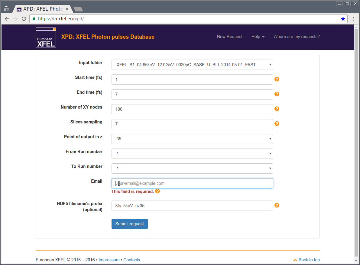
Provide your email address and click "Submit request". A pop-up window will open displaying a request ID and an url. This url will point to a website where the status of the request can be checked. At the same website a zip file with the data can be downloaded once the job is done. Download and extract this zip file to a place of your liking.
In the following, we will assume that the file was extracted to directory "source/" in the working directory and is named "3fs_5keV_nz35_0000001.h5".
Propagation of x-ray pulses through the SPB-SFX beamline will be performed by means of the
SimEx.Calculators.XFELPhotonPropagator.XFELPhotonPropagator class (see API: XFELPhotonPropagator), that comes with simex_platform. It interfaces the wavefront propagation code WPG.
A documented python script demonstrates the wavefront propagation:
It loads a WPG beamline from the beamline collection in folder ./lib/python2.7/prop of your simex_platform installation. The variable input_files_path needs to be adjusted before executing the script. It should contain a path pointing at the source files you downloaded in the previous section (see Preparing the source input). It can be either a file or a directory. In the latter case, all valid source files in the directory will be processed.
The XFELPhotonPropagator class requires two input parameters, a parameters object of type SimEx.Parameters.WavePropagatorParameters.WavePropagatorParameters (WavePropagatorParameters), and the input_path. After construction, the input files are read in using the method _readH5 and the calculation is executed by calling the backengine (backengine) method.
A third input parameter for the XFELPhotonPropagator class, output_path can be used to specify where the results of the wavefront propagation shall be saved. By default, they are stored in a directory called "prop/" below the current working directory.
Please notice that the execution of the backengine method might take a while. Furthermore, some exceptions might be displayed which do not influence the final output.
Confirm that the results of the wavefront propagation are saved to "prop/". The script prop_diagnostics.py provides utilities to quickly diagnose single propagated x-ray pulses. The syntax is:
$> prop_diagnostics.py <options> prop_out.h5
Running prop_diagnostics.py without arguments will return a small instruction how to use it.
E.g.:
$> prop_diagnostics.py -I prop_out.h5
generates an intensity map of the radiation field in the focus. Likewise,:
$> prop_diagnostics.py -R prop_out.h5
plots the intensity distribution in reciprocal (qx-qy) space.
The options -T, -X, -S produce viewgraphs of the total power as function of time, the on-axis power as function of time,
and the power spectrum as a function of photon energy, respectively.
Running the script on the source file:
$> prop_diagnostics.py <options> source/s2e_felsource.h5
will produce the same figures for the source. Comparison of source and propagated pulses can give some information about the reliability of the propagation. E.g. a drastic loss in power would indicate that the area over which the wavefront was calculated, is too small or that the wavefront is insufficiently sampled. The resulting graphs should look similar to these:
FEL power (averaged over x,y coordinates) as function of time, source (left) vs. focus (right):

FEL on-axis power density as function of time, source (left) vs. focus (right):

Intensity distribution, source (left) vs. focus (right):

Intensity distribution in reciprocal space, source (left) vs. focus (right):

Confirm that the pulse duration is approximately 9 fs (full width at half maximum, FWHM), that the focus has a FWHM of approximately 100 nm and as well as that the reciprocal intensity distribution is smooth and shows no artificial high frequency modes.
The simex_platform employs the atomistic simulation codes XMDYN and XATOM to simulate
the interaction of the sample with the x-ray pulse. Unfortunately, these codes are not Open Source
and simex_platform only provides a demo version of the code. The corresponding Calculator is the
XSimEx.Calculators.XMDYNDemoPhotonMatterInteractor.XMDYNDemoPhotonMatterInteractor (see API: XMDYNDemoPhotonMatterInteractor).
To simulate the photon-matter interaction the script pmi.py can be used. It shows how to use the XMDYNDemoPhotonMatterInteractor to produce photon-matter trajectories which will then be used to calculate the diffraction.
For the simulation of the interaction the protein nitrogenase iron protein from Azotobacter Vinelandii (see 2NIP at Protein Data Base ) is used. You can download the pdb file from this link or simex_platform will do it for you if it cannot find the file 2NIP.pdb in the path specified by the 'sample_path' argument of XMDYNDemoPhotonMatterInteractor.__init__(...).
Let's take a look at the results of the photon matter interaction calculation. The script pmi_diagnostics.py plots the average number of bound electrons per atom species in the sample and the average displacement as a function of time. To get to the manual site, type:
$> pmi_diagnostics.py
Alternatively, ipython can be used:
$> ipython
In ipython the following lines can be executed:
>import numpy as np

>import matplotlib.pyplot as plt

>run <path to simex_platform>/Sources/python/ScriptCollection/DataAnalysis/pmi/pmi_diagnostics.py

>data=pmi_diagnostics('load',[1],np.arange(1,11))
This will load the file in ./pmi/ and selects 10 snapshots. If there are more input files in the ./pmi folder you can change [1] to [1,2,3,...,n].
Since this is the demo version of the pmi code, the results are pretty boring, since no radiation damage happens, neither ionization nor atomic displacement.
The next step is to calculate the diffraction of photons from the sample as it is exposed to the beam, i.e. radiation damage and diffraction or scattering happen simultaneously. In the previous section, we have pre-calculated the atomic structure (atom positions as a function of time) and the electronic structure as a function of time. Based on this information we can now proceed to calculate the amount of scattered radiation into a given detector pixel as a function of time. The detector signal will then be calculated by integrating over the exposure time or pulse duration, whichever is shorter.
We use SimEx.Calculators.SingFELPhotonDiffractor.SingFELPhotonDiffractor (see API: SingFELPhotonDiffractor). The script demonstrating it's usage can be copied from diffraction.py.
The parameter files that describe the beam can be copied from s2e.beam and s2e.geom. Please copy them to your local folder.
Run the script diffr_diagnostics.py to generate statistical information about the number of scattered photons and a histogram. Envoke the script without any arguments to get obtain usage instructions.
For example:
$> diffr_diagnostics.py -p 1 -P ./diffr/<filename>.h5
will show the detected photons in the detector pixel array for the first pattern.
A more complicated example is:
$> diffr_diagnostics.py -p "range(1,11)" -P --logscale --operation "numpy.mean" ./diffr/<filename>.h5
this will plot the average detector image on a logarithmic color scale for patterns 1 through 10. Keep in mind that the default numbering of patterns starts off with 1 (hdf group 0000001).
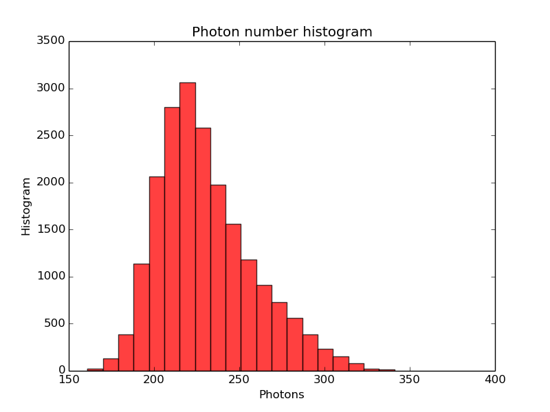
To see a histogram over the number of photons per pattern:
$> diffr_diagnostics.py -S "range(1,11)" -P ./diffr/<filename>.h5
To create an animation of all selected patterns:
$> diffr_diagnostics.py -A animation.gif "range(1,11)" -P ./diffr/<filename>.h5
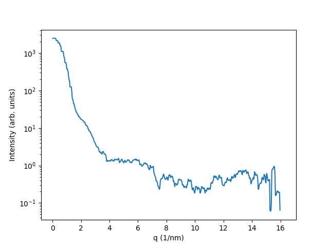
The flag -R triggers generation of a radial intensity profile using azimuthal integration (with pyFAI). This can easily be used to synthesize a SAXS signal by combining summation and azimuthal integration:
$> diffr_diagnostics.py -P -R -l -o "numpy.sum" ./diffr/<filename>.h5
which results in a plot similar to this: