readme.md

Disjoint Set Union / Union find

A disjoint-set data structure is defined as a data structure that keeps track of a set of elements partitioned into a number of disjoint (non-overlapping) subsets.

• Disjoint Set: Two sets are called disjoint set if the intersection of two sets is \phiϕ i.e. NULL. A Disjoint-Set data structure that keeps records of a set of elements partitioned into several non-overlapping (Disjoint) subsets.

A DSU will have an operation to combine any two sets, and it will be able to tell in which set a specific element is. The classical version also introduces a third operation, it can create a set from a new element.

Thus the basic interface of this data structure consists of only three operations:

• make_set(v) - creates a new set consisting of the new element v
• union_sets(a, b) - merges the two specified sets (the set in which the element a is located, and the set in which the element b is located)
• find_set(v) - returns the representative (also called leader) of the set that contains the element v. This representative is an element of its corresponding set. It is selected in each set by the data structure itself (and can change over time, namely after union_sets calls). This representative can be used to check if two elements are part of the same set or not. a and b are exactly in the same set, if find_set(a) == find_set(b). Otherwise they are in different sets.

Disjoint Set Union is sometimes also referred to as Union-Find because of its two important operations :

Union-Find algorithm performs two very useful operations -

• Find: To find the subset a particular element 'k' belongs to. It is generally used to check if two elements belong to the same subset or not.

• Union: It is used to combine two subsets into one. A union query, say Union(x, y) combines the set containing element x and set containing element y.

Construction of Efficient Data Structure :

We will store the sets in the form of trees: each tree will correspond to one set. And the root of the tree will be the representative/leader of the set.

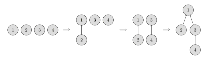
In the beginning, every element starts as a single set, therefore each vertex is its own tree. Then we combine the set containing the element 1 and the set containing the element 2. Then we combine the set containing the element 3 and the set containing the element 4. And in the last step, we combine the set containing the element 1 and the set containing the element 3.

For the implementation this means that we will have to maintain an array parent that stores a reference to its immediate ancestor in the tree.

Naive Implementation :

• All the information about the sets of elements will be kept in an array parent.
• To create a new set (operation make_set(v)), we simply create a tree with root in the vertex v, meaning that it is its own ancestor.
• To combine two sets (operation union_sets(a, b)), we first find the representative of the set in which a is located, and the representative of the set in which b is located.
• If the representatives are identical, that we have nothing to do, the sets are already merged. Otherwise, we can simply specify that one of the representatives is the parent of the other representative - thereby combining the two trees.
• Finally the implementation of the find representative function (operation find_set(v)): we simply climb the ancestors of the vertex v until we reach the root, i.e. a vertex such that the reference to the ancestor leads to itself. This operation is easily implemented recursively.

Code :

void make_set(int v) {
    parent[v] = v;
}

int find_set(int v) {
    if (v == parent[v])
        return v;
    return find_set(parent[v]);
}

void union_sets(int a, int b) {
    a = find_set(a);
    b = find_set(b);
    if (a != b)
        parent[b] = a;
}

Note : However this implementation is inefficient. It is easy to construct an example, so that the trees degenerate into long chains. In that case each call find_set(v) can take O(n) time.

Path compression optimization :

• This optimization is designed for speeding up find_set.
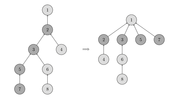
• If we call find_set(v) for some vertex v, we actually find the representative p for all vertices that we visit on the path between v and the actual representative p. The trick is to make the paths for all those nodes shorter, by setting the parent of each visited vertex directly to p.
• You can see the operation in the following image. On the left there is a tree, and on the right side there is the compressed tree after calling find_set(7), which shortens the paths for the visited nodes 7, 5, 3 and 2.

Optimized code of find_set :

int find_set(int v) {
    if (v == parent[v])
        return v;
    return parent[v] = find_set(parent[v]);
}

Union by size / rank :

• In this optimization we will change the union_set operation.
• There are two approaches :
  • In the first approach we use the size of the trees as rank.
  • In the second one we use the depth of the tree (more precisely, the upper bound on the tree depth, because the depth will get smaller when applying path compression).
• In both approaches the essence of the optimization is the same: we attach the tree with the lower rank to the one with the bigger rank.

Optimized code for union_set :

• Union by size

void make_set(int v) {
    parent[v] = v;
    size[v] = 1;
}

void union_sets(int a, int b) {
    a = find_set(a);
    b = find_set(b);
    if (a != b) {
        if (size[a] < size[b])
            swap(a, b);
        parent[b] = a;
        size[a] += size[b];
    }
}

• Union by rank based on the depth of the trees

void make_set(int v) {
    parent[v] = v;
    rank[v] = 0;
}

void union_sets(int a, int b) {
    a = find_set(a);
    b = find_set(b);
    if (a != b) {
        if (rank[a] < rank[b])
            swap(a, b);
        parent[b] = a;
        if (rank[a] == rank[b])
            rank[a]++;
    }
}

Both optimizations are equivalent in terms of time and space complexity. So in practice you can use any of them.

Time Complexity :

Time complexity of an algorithm quantifies the amount of time taken by an algorithm to run as a function of the length of the input. Time complexity is commonly estimated by counting the number of elementary operations performed by the algorithm, supposing that each elementary operation takes a fixed amount of time to perform.

The final amortized time complexity is ~O(4*n).

Applications :

• It is used to find Cycle in a graph as in Kruskal's algorithm, DSUs are used.
• Checking for connected components in a graph.
• Searching for connected components in an image.
• Offline LCA (lowest common ancestor in a tree)
• Offline RMQ (range minimum query) / Arpa's trick