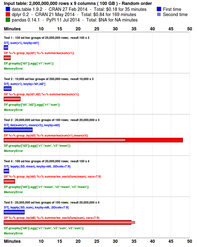
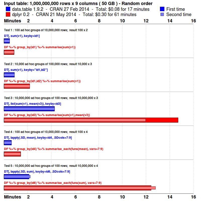
Benchmarks : Grouping

• The input data is randomly ordered. No pre-sort. No indexes. No key.
• 5 simple queries are run. Similar to what a data analyst might do in practice; i.e., various ad hoc aggregations as the data is explored and investigated.
• Each package is tested separately in its own fresh R session.
• Each query is repeated once more, immediately. This is to isolate cache effects and confirm the first timing. The first and second times are plotted. The total runtime is also displayed.
• The results are compared and checked allowing for numeric tolerance and column name differences.

Scroll down to find reproducible code, system info and FAQ.

---

Smaller tests : 1E7 1E8 1E9

Code to reproduce the timings above :

## data.table run
$ R --vanilla
require(data.table)
N=2e9; K=100
set.seed(1)
DT <- data.table(
  id1 = sample(sprintf("id%03d",1:K), N, TRUE),      # large groups (char)
  id2 = sample(sprintf("id%03d",1:K), N, TRUE),      # large groups (char)
  id3 = sample(sprintf("id%010d",1:(N/K)), N, TRUE), # small groups (char)
  id4 = sample(K, N, TRUE),                          # large groups (int)
  id5 = sample(K, N, TRUE),                          # large groups (int)
  id6 = sample(N/K, N, TRUE),                        # small groups (int)
  v1 =  sample(5, N, TRUE),                          # int in range [1,5]
  v2 =  sample(5, N, TRUE),                          # int in range [1,5]
  v3 =  sample(round(runif(100,max=100),4), N, TRUE) # numeric e.g. 23.5749
)
cat("GB =", round(sum(gc()[,2])/1024, 3), "\n")
system.time( DT[, sum(v1), keyby=id1] )
system.time( DT[, sum(v1), keyby=id1] )
system.time( DT[, sum(v1), keyby="id1,id2"] )
system.time( DT[, sum(v1), keyby="id1,id2"] )
system.time( DT[, list(sum(v1),mean(v3)), keyby=id3] )
system.time( DT[, list(sum(v1),mean(v3)), keyby=id3] )
system.time( DT[, lapply(.SD, mean), keyby=id4, .SDcols=7:9] )
system.time( DT[, lapply(.SD, mean), keyby=id4, .SDcols=7:9] )
system.time( DT[, lapply(.SD, sum), keyby=id6, .SDcols=7:9] )
system.time( DT[, lapply(.SD, sum), keyby=id6, .SDcols=7:9] )

## dplyr run
$ R --vanilla
require(dplyr)
N=2e9; K=100
set.seed(1)
DF <- data.frame(stringsAsFactors=FALSE,
  id1 = sample(sprintf("id%03d",1:K), N, TRUE),
  id2 = sample(sprintf("id%03d",1:K), N, TRUE),
  id3 = sample(sprintf("id%010d",1:(N/K)), N, TRUE),
  id4 = sample(K, N, TRUE),                          
  id5 = sample(K, N, TRUE),                         
  id6 = sample(N/K, N, TRUE),                       
  v1 =  sample(5, N, TRUE),                         
  v2 =  sample(1e6, N, TRUE),                       
  v3 =  sample(round(runif(100,max=100),4), N, TRUE)
)
cat("GB =", round(sum(gc()[,2])/1024, 3), "\n")
system.time( DF %>% group_by(id1) %>% summarise(sum(v1)) )
system.time( DF %>% group_by(id1) %>% summarise(sum(v1)) )
system.time( DF %>% group_by(id1,id2) %>% summarise(sum(v1)) )
system.time( DF %>% group_by(id1,id2) %>% summarise(sum(v1)) )
system.time( DF %>% group_by(id3) %>% summarise(sum(v1),mean(v3)) )
system.time( DF %>% group_by(id3) %>% summarise(sum(v1),mean(v3)) )
system.time( DF %>% group_by(id4) %>% summarise_each(funs(mean), vars=7:9) )
system.time( DF %>% group_by(id4) %>% summarise_each(funs(mean), vars=7:9) )
system.time( DF %>% group_by(id6) %>% summarise_each(funs(sum), vars=7:9) )
system.time( DF %>% group_by(id6) %>% summarise_each(funs(sum), vars=7:9) )

R info

$ R --vanilla
# R version 3.1.1 (2014-07-10) -- "Sock it to Me"
# Copyright (C) 2014 The R Foundation for Statistical Computing
# Platform: x86_64-pc-linux-gnu (64-bit)

> sessionInfo()
# R version 3.1.1 (2014-07-10)
# Platform: x86_64-pc-linux-gnu (64-bit)
# 
# locale:
#  [1] LC_CTYPE=en_US.UTF-8       LC_NUMERIC=C
#  [3] LC_TIME=en_US.UTF-8        LC_COLLATE=en_US.UTF-8
#  [5] LC_MONETARY=en_US.UTF-8    LC_MESSAGES=en_US.UTF-8
#  [7] LC_PAPER=en_US.UTF-8       LC_NAME=C
#  [9] LC_ADDRESS=C               LC_TELEPHONE=C
# [11] LC_MEASUREMENT=en_US.UTF-8 LC_IDENTIFICATION=C

# attached base packages:
# [1] stats     graphics  grDevices utils     datasets  methods base

# other attached packages:
# [1] dplyr_0.2        data.table_1.9.2
# 
# loaded via a namespace (and not attached):
# [1] assertthat_0.1 parallel_3.1.1 plyr_1.8.1     Rcpp_0.11.2 reshape2_1.4
# [6] stringr_0.6.2  tools_3.1.1

System info

Amazon EC2 r3.8large

$ lsb_release -a
# No LSB modules are available.
# Distributor ID:    Ubuntu
# Description:    Ubuntu 14.04 LTS
# Release:    14.04
# Codename:    trusty

$ uname -a
# Linux ip-172-31-33-222 3.13.0-29-generic #53-Ubuntu SMP
# Wed Jun 4 21:00:20 UTC 2014 x86_64 x86_64 x86_64 GNU/Linux

$ lscpu
# Architecture:          x86_64
# CPU op-mode(s):        32-bit, 64-bit
# Byte Order:            Little Endian
# CPU(s):                32
# On-line CPU(s) list:   0-31
# Thread(s) per core:    2
# Core(s) per socket:    8
# Socket(s):             2
# NUMA node(s):          2
# Vendor ID:             GenuineIntel
# CPU family:            6
# Model:                 62
# Stepping:              4
# CPU MHz:               2494.090
# BogoMIPS:              5049.01
# Hypervisor vendor:     Xen
# Virtualization type:   full
# L1d cache:             32K
# L1i cache:             32K
# L2 cache:              256K
# L3 cache:              25600K
# NUMA node0 CPU(s):     0-7,16-23
# NUMA node1 CPU(s):     8-15,24-31

$ free -h
#              total       used       free     shared    buffers cached
# Mem:          240G       2.4G       237G       364K        60M 780M
# -/+ buffers/cache:       1.6G       238G
# Swap:           0B         0B         0B

FAQ

What about compiler flags?

R by default compiles packages with -g -O2. There are some known problems with -O3 with some packages in some circumstances so that decision is not an oversight. On the other hand we don't fully understand which packages are affected and to what degree. So for these benchmarks, we do install with the following in ~/.R/Makevars :

CFLAGS=-O3 -mtune=native
CXXFLAGS=-O3 -mtune=native

This can speed up by up to 30%; e.g., see tests 3 and 5 in before and after plots below. Right click and 'open image in a new tab' to see these images full size. [We realise a single chart showing the percentage change would be better, but not a priority. We'll just go ahead with -O3 to isolate that concern.]

Why not a single line chart rather than multiple bar plots for each size?

Because we want to compare syntax too. The syntax is quite wide so a horizontal bar chart accommodates that text. The image can grow in height as more tests or packages are added whereas a line chart starts to become cluttered. The largest size is likely the most interesting; we don't expect many people to look at the smaller sizes.

Shouldn't there be a gc() between each system.time()?

system.time() already does that built-in. It has a gcFirst argument, by default TRUE. The time for that gc is excluded by system.time.

Those costs are tiny. Are they the EC2 compute cost?

Yes @ $0.30/hour as a spot instance. The machine specs are above. It was just to show how accessible and cheap large RAM on-demand machines can be.

What about comparing memory usage too?

Yes we'd like to but didn't know how to measure that via the command line. This looks perfect: https://github.com/gsauthof/cgmemtime.

Does either package have a parallel option?

Not currently. There are 32 CPU's on this machine and only one is being used, so that's an obvious thing to address.

How does SQL compare?

We'll try and test. Contributed tests are more than welcome.

Is dplyr faster with a database backend?

Likely it depends on which database backend. Feel like testing it?

How does Python's Pandas compare?

We are testing it, results soon.

Has anything else changed?

v2 was originally sample(1e6, N, TRUE) but the size of these ints caused sum(v2) in test 5 to overflow. R detects this and coerces to numeric. To keep things simple we changed it to sample(5, N, TRUE) just like v1.

Why do the data.table commands use keyby= rather than by=?

To match dplyr. by= in data.table returns the groups in the order they first appear in the dataset. (Apparently, Stata also has this feature.) It can be important when the data is grouped in blocks and the order those blocks appear has some meaning. But as far as we know dplyr has no equivalent; it always sorts the returned groups. keyby= is a by= followed by a setkey on the group columns in the result.

Why did you run these benchmarks?

To know what the facts are and to demonstrate what we think a decent benchmark for large data is. Also to gain feedback and ideas for improvement.

Is 2 billion the limit?

Yes. data.table and we believe data.frame are both currently limited to 2^31 rows. To increase this limit we need to start using long vectors internally which were new in R 3.0.

Why just grouping?

Because we had to start somewhere. Joins and updates will follow.

Is just testing sum and mean too simple?

Yes probably, but we had to start somewhere. sum and mean benefit from advanced optimizations in both packages. Adding, say, median is expected to give different results. As might sum()+1 and other expressions that may be more difficult to optimize.

Is it elapsed time that's measured?

Strictly speaking, it's user+sys. Other unrelated tasks on the machine can affect elapsed, we believe. However, this server had so many CPUs and so much memory that elapsed==user+sys in all cases.

What if the groups aren't randomly shuffled but there's some clustering?

Good question. All packages should be faster due to better cache efficiency. Some may benefit more than others and it'd be great to do that. Any volunteers? However, a feature of this benchmark is that it's a sum of 5 different queries. In real life, if groups are clustered then it can only be on one dimension (e.g. (id,time) or (time,id), but not both). We're trying to capture that with this benchmark.

How about -flto and similar extra flags?

If there's evidence that it's worth the testing time we're happy to do so. Is there any downside to the extra flag? Why haven't the compiler developers included it in -O3 already? It's a complicated topic; e.g. What are your compiler flags?.

Base R's mean accumulates in long double precision where the machine supports it (and most do) and then does a second pass through the entire vector to adjust mean(x) by typically a very small amount to ensure that sum(x-mean(x)) is minimized. What do these packages do?

Both data.table and dplyr currently do a single pass sum(x)/length(x) where the sum is done in long double precision. They match base in terms of long double but don't do the second pass, currently. Feedback welcome.

What about base R grouping functions?

It would be great to add a comparison for 1E7 rows. We expect the scale to be hours or possibly days for 2E9.

Why haven't the faster methods been incorporated into R itself?

• data.table and dplyr are still developing and not yet fully mature
• as you can see from the answer about mean above, they are sometimes not precisely the same as base R. This is the same reason fread hasn't replaced read.csv, because it isn't yet a drop in replacement (ability to read from connections being the main difference).
• it isn't just speed but both packages prefer a different syntax to base R
• a lot of new code at C level would need to be added to R itself and a large amount of testing and risk of breakage (5,000 dependent packages on CRAN). To date there hasn't been the will or the time.
• packages are a fantastic way to allow progress without breaking base R and its dependants.

Have all these questions really been asked?

Yes they have. Even this question was asked. This is why this is a wiki page, so we could improve the benchmark and easily add to this FAQ as comments and suggestions come in.

How do I contact you?

Matt Dowle; mdowle at mdowle.plus.com